how to find average rate of change on a graph

Learning Objectives

In this section, you will:

• Find the boilerplate rate of change of a function.
• Use a graph to determine where a role is increasing, decreasing, or constant.
• Apply a graph to locate local maxima and local minima.
• Use a graph to locate the accented maximum and absolute minimum.

Gasoline costs have experienced some wild fluctuations over the last several decades. (Effigy)^[one] lists the average cost, in dollars, of a gallon of gasoline for the years 2005–2012. The cost of gasoline tin be considered as a function of twelvemonth.

If we were interested merely in how the gasoline prices changed between 2005 and 2022, we could compute that the toll per gallon had increased from $ii.31 to $iii.68, an increase of $i.37. While this is interesting, it might be more useful to look at how much the price inverse per year. In this section, we will investigate changes such as these.

Finding the Boilerplate Rate of Change of a Function

The price alter per year is a charge per unit of modify because it describes how an output quantity changes relative to the change in the input quantity. Nosotros can encounter that the price of gasoline in (Figure) did not change by the aforementioned amount each year, then the rate of change was non constant. If nosotros use merely the commencement and ending information, nosotros would exist finding the boilerplate charge per unit of change over the specified catamenia of time. To find the average charge per unit of change, we split up the change in the output value by the alter in the input value.

[latex]\begin{array}{ccc}\hfill \text{Boilerplate rate of change}& =& \frac{\text{Change in output}}{\text{Change in input}}\hfill \\ & =& \frac{\Delta y}{\Delta 10}\hfill \\ & =& \frac{{y}_{two}-{y}_{i}}{{x}_{ii}-{x}_{1}}\hfill \\ & =& \frac{f\left({x}_{2}\right)-f\left({x}_{1}\correct)}{{x}_{ii}-{x}_{one}}\hfill \end{array}[/latex]

The Greek alphabetic character[latex]\text{Δ}\,[/latex](delta) signifies the change in a quantity; we read the ratio as "delta-y over delta-ten" or "the change in[latex]\,y\,[/latex]divided by the alter in[latex]\,x.[/latex]" Occasionally we write[latex]\,\text{Δ}f\,[/latex]instead of[latex]\,\text{Δ}y,\,[/latex]which still represents the change in the function'southward output value resulting from a alter to its input value. It does not mean we are irresolute the office into some other function.

In our instance, the gasoline cost increased past $ane.37 from 2005 to 2022. Over 7 years, the average rate of change was

[latex]\frac{\text{Δ}y}{\text{Δ}x}=\frac{\text{\$}one.37}{\text{7 years}}\approx 0.196\text{ dollars per year}[/latex]

On boilerplate, the price of gas increased by about 19.6¢ each year.

Other examples of rates of change include:

• A population of rats increasing by 40 rats per calendar week
• A car traveling 68 miles per hr (distance traveled changes past 68 miles each hour equally time passes)
• A automobile driving 27 miles per gallon (distance traveled changes by 27 miles for each gallon)
• The current through an electrical circuit increasing by 0.125 amperes for every volt of increased voltage
• The amount of money in a college account decreasing by $4,000 per quarter

Charge per unit of Change

A rate of change describes how an output quantity changes relative to the change in the input quantity. The units on a rate of change are "output units per input units."

The average rate of change between two input values is the total modify of the function values (output values) divided by the change in the input values.

[latex]\frac{\Delta y}{\Delta x}=\frac{f\left({x}_{2}\right)-f\left({x}_{1}\right)}{{ten}_{2}-{ten}_{1}}[/latex]

How To

Given the value of a part at different points, calculate the average rate of change of a part for the interval between two values[latex]\,{x}_{one}\,[/latex]and[latex]\,{x}_{2}.[/latex]

1. Summate the difference [latex]{y}_{2}-{y}_{1}=\text{Δ}y.[/latex]
2. Summate the difference [latex]{ten}_{2}-{ten}_{ane}=\text{Δ}ten.[/latex]
3. Observe the ratio[latex]\,\frac{\text{Δ}y}{\text{Δ}10}.[/latex]

Computing an Average Rate of Modify

Using the information in (Figure), find the average rate of alter of the price of gasoline between 2007 and 2009.

Analysis

Annotation that a decrease is expressed by a negative change or "negative increase." A rate of change is negative when the output decreases every bit the input increases or when the output increases as the input decreases.

Endeavor It

Using the data in (Figure), find the boilerplate charge per unit of alter betwixt 2005 and 2022.

Prove Solution

[latex]\frac{$2.84-$2.31}{5\text{ years}}=\frac{\$0.53}{v\text{ years}}=$0.106\,[/latex]per year.

Calculating Boilerplate Rate of Change from a Graph

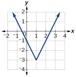
Given the office[latex]\,g\left(t\right)\,[/latex]shown in (Figure), find the average rate of change on the interval[latex]\,\left[-i,two\right].[/latex]

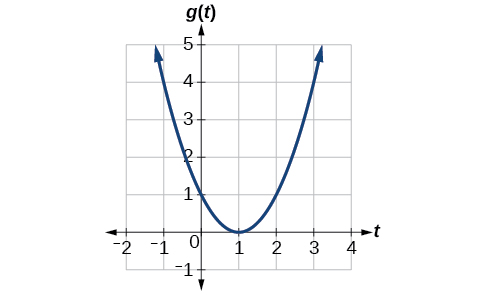
Figure 1.

Analysis

Notation that the order we choose is very important. If, for case, nosotros use[latex]\,\frac{{y}_{2}-{y}_{1}}{{x}_{ane}-{ten}_{ii}},\,[/latex]we volition not become the correct answer. Determine which point will be one and which point will be two, and keep the coordinates stock-still as[latex]\,\left({10}_{i},{y}_{ane}\right)\,[/latex]
and[latex]\,\left({x}_{2},{y}_{2}\correct).[/latex]

Calculating Boilerplate Charge per unit of Change from a Table

After picking up a friend who lives 10 miles abroad and leaving on a trip, Anna records her distance from domicile over time. The values are shown in (Figure). Find her average speed over the first 6 hours.

t (hours)	0	1	two	iii	4	5	half dozen	vii
D(t) (miles)	10	55	xc	153	214	240	292	300

Analysis

Considering the speed is non constant, the average speed depends on the interval called. For the interval [two,3], the boilerplate speed is 63 miles per 60 minutes.

Computing Boilerplate Rate of Alter for a Role Expressed every bit a Formula

Compute the average rate of alter of [latex]f\left(x\right)={x}^{two}-\frac{1}{x}[/latex] on the interval [latex]\text{[two,}\,\text{4].}[/latex]

Try Information technology

Observe the boilerplate rate of change of [latex]f\left(10\correct)=x-2\sqrt{10}[/latex] on the interval [latex]\left[i,\,9\right].[/latex]

Show Solution

[latex]\frac{1}{2}[/latex]

Finding the Average Rate of Change of a Strength

The electrostatic force[latex]\,F,[/latex]measured in newtons, between two charged particles can exist related to the altitude between the particles[latex]\,d,[/latex]in centimeters, by the formula[latex]\,F\left(d\right)=\frac{2}{{d}^{two}}.[/latex]Notice the average charge per unit of change of force if the distance between the particles is increased from 2 cm to 6 cm.

Finding an Average Rate of Change as an Expression

Observe the average charge per unit of modify of [latex]grand\left(t\correct)={t}^{2}+3t+1[/latex] on the interval [latex]\left[0,\,a\correct].[/latex] The reply will be an expression involving [latex]a[/latex] in simplest form.

Try It

Discover the average rate of change of[latex]\,f\left(10\right)={10}^{2}+2x-8\,[/latex] on the interval[latex]\,\left[5,a\right]\,[/latex]in simplest forms in terms

Evidence Solution

[latex]\,a+seven\,[/latex]

Using a Graph to Determine Where a Function is Increasing, Decreasing, or Constant

Every bit part of exploring how functions change, we can place intervals over which the function is changing in specific ways. Nosotros say that a function is increasing on an interval if the office values increment every bit the input values increase within that interval. Similarly, a function is decreasing on an interval if the office values decrease as the input values increment over that interval. The boilerplate charge per unit of change of an increasing function is positive, and the average rate of change of a decreasing function is negative. (Figure) shows examples of increasing and decreasing intervals on a function.

Figure 3. The function[latex]\,f\left(10\correct)={x}^{3}-12x\,[/latex]is increasing on[latex]\,\left(-\infty \text{,}\,-\text{two}\right){{\cup }^{\text{​}}}^{\text{​}}\left(2,\,\infty \right)\,[/latex]and is decreasing on[latex]\,\left(-2\text{,}\,2\right).[/latex]

While some functions are increasing (or decreasing) over their entire domain, many others are not. A value of the input where a function changes from increasing to decreasing (as we go from left to right, that is, every bit the input variable increases) is chosen a local maximum. If a role has more than i, we say it has local maxima. Similarly, a value of the input where a function changes from decreasing to increasing as the input variable increases is chosen a local minimum. The plural form is "local minima." Together, local maxima and minima are chosen local extrema, or local farthermost values, of the office. (The singular form is "extremum.") Often, the term local is replaced by the term relative. In this text, nosotros will use the term local.

Clearly, a part is neither increasing nor decreasing on an interval where it is abiding. A role is also neither increasing nor decreasing at extrema. Notation that nosotros have to speak of local extrema, because any given local extremum every bit defined here is not necessarily the highest maximum or everyman minimum in the office's entire domain.

For the part whose graph is shown in (Effigy), the local maximum is 16, and it occurs at[latex]\,x=-2.\,[/latex]The local minimum is[latex]\,-16\,[/latex]and it occurs at[latex]\,x=2.[/latex]

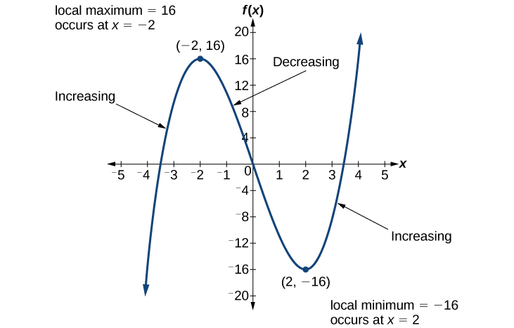
Figure four.

To locate the local maxima and minima from a graph, nosotros need to detect the graph to determine where the graph attains its highest and everyman points, respectively, inside an open up interval. Like the acme of a roller coaster, the graph of a role is higher at a local maximum than at nearby points on both sides. The graph volition also be lower at a local minimum than at neighboring points. (Figure) illustrates these ideas for a local maximum.

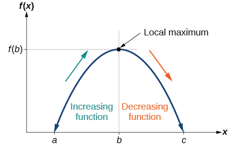
Figure 5. Definition of a local maximum

These observations lead us to a formal definition of local extrema.

Local Minima and Local Maxima

A function[latex]\,f\,[/latex]is an increasing function on an open interval if[latex]\,f\left(b\right)>f\left(a\right)\,[/latex]for any two input values[latex]\,a\,[/latex]and[latex]\,b\,[/latex]in the given interval where[latex]\,b>a.[/latex]

A part[latex]\,f\,[/latex]is a decreasing function on an open interval if[latex]\,f\left(b\right)<f\left(a\right)\,[/latex]for whatever two input values[latex]\,a\,[/latex]and[latex]\,b\,[/latex]in the given interval where[latex]\,b>a.[/latex]

A role [latex]f[/latex] has a local maximum at [latex]\,x=b[/latex] if there exists an interval [latex]\,\left(a,c\right)[/latex] with [latex]a<b<c[/latex] such that, for whatsoever [latex]x[/latex] in the interval[latex]\left(a,c\correct),[/latex][latex]f\left(10\right)\le f\left(b\right).[/latex] Likewise, [latex]f[/latex] has a local minimum at [latex]ten=b[/latex] if there exists an interval [latex]\left(a,c\correct)[/latex] with [latex]a<b<c[/latex] such that, for any [latex]x[/latex] in the interval [latex]\left(a,c\right),[/latex][latex]f\left(x\correct)\ge f\left(b\right).[/latex]

Finding Increasing and Decreasing Intervals on a Graph

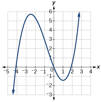
Given the function[latex]\,p\left(t\correct)\,[/latex]in (Figure), place the intervals on which the part appears to be increasing.

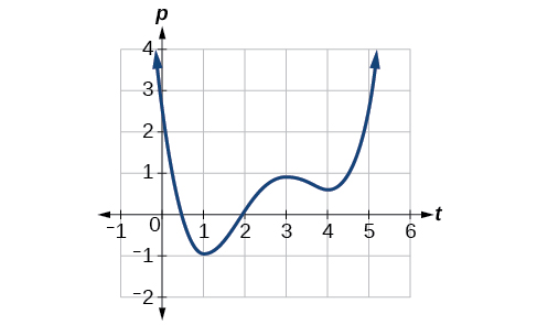
Effigy half dozen.

Analysis

Observe in this example that we used open up intervals (intervals that do not include the endpoints), because the part is neither increasing nor decreasing at[latex]\,t=1[/latex],[latex]\,t=3[/latex], and[latex]\,t=4\,[/latex]. These points are the local extrema (ii minima and a maximum).

Finding Local Extrema from a Graph

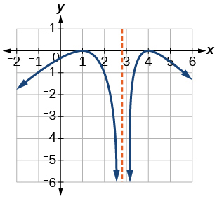
Graph the function[latex]\,f\left(x\correct)=\frac{2}{x}+\frac{ten}{3}.\,[/latex]Then use the graph to estimate the local extrema of the function and to decide the intervals on which the function is increasing.

Analysis

Most graphing calculators and graphing utilities tin gauge the location of maxima and minima. (Figure) provides screen images from two unlike technologies, showing the judge for the local maximum and minimum.

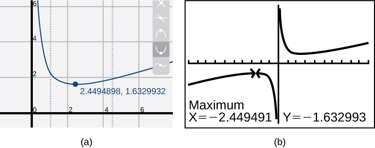
Effigy 8.

Based on these estimates, the role is increasing on the interval[latex]\,(-\infty \text{,}-\text{2}\text{.449)}\,[/latex]
and[latex]\,\left(2.449\text{,}\infty \right).\,[/latex]Find that, while we look the extrema to be symmetric, the two different technologies agree only up to four decimals due to the differing approximation algorithms used by each. (The verbal location of the extrema is at[latex]\,±\sqrt{half dozen},\,[/latex]but determining this requires calculus.)

Endeavor Information technology

Graph the function[latex]\,f\left(ten\right)={ten}^{3}-6{x}^{two}-15x+xx\,[/latex]to estimate the local extrema of the function. Utilise these to determine the intervals on which the function is increasing and decreasing.

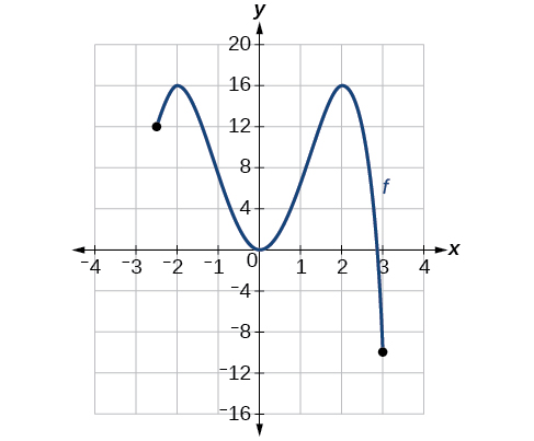
Finding Local Maxima and Minima from a Graph

For the function[latex]\,f\,[/latex]whose graph is shown in (Figure), find all local maxima and minima.

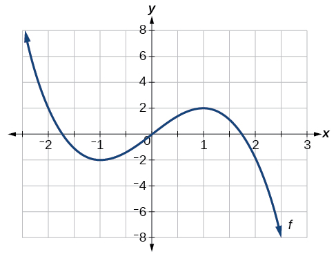
Figure 9

Analyzing the Toolkit Functions for Increasing or Decreasing Intervals

We volition now return to our toolkit functions and talk over their graphical behavior in (Figure), (Figure), and (Figure).

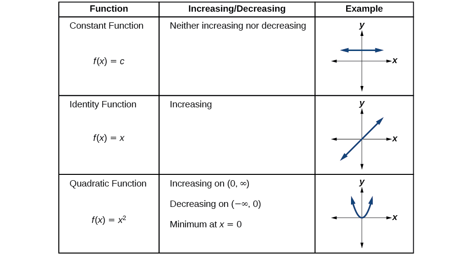
Figure 10.

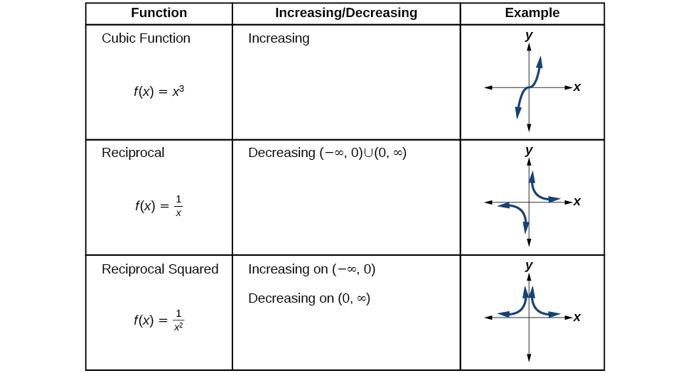
Figure xi.

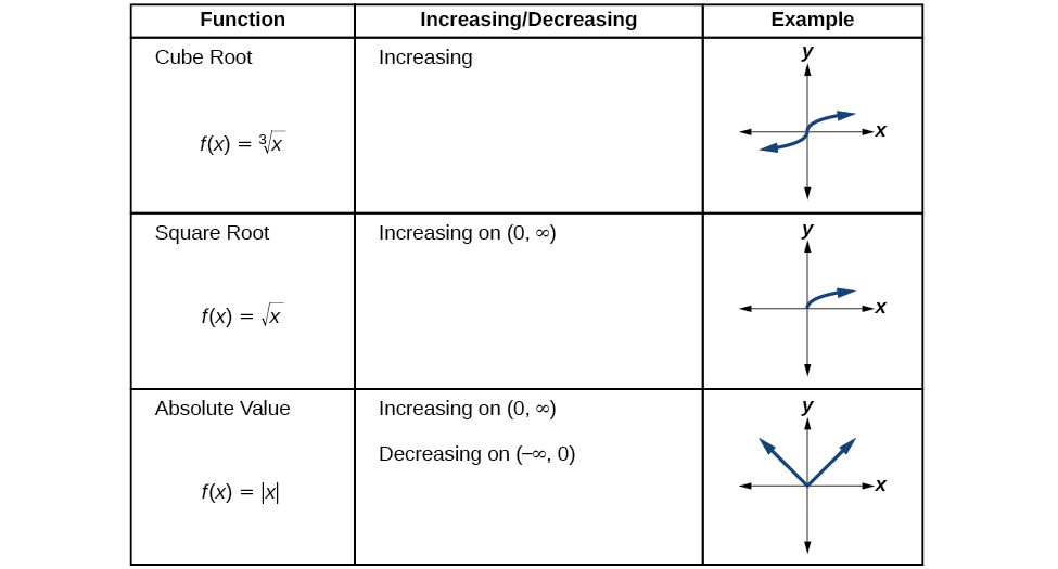
Figure 12.

Utilise A Graph to Locate the Accented Maximum and Absolute Minimum

There is a difference between locating the highest and lowest points on a graph in a region around an open up interval (locally) and locating the highest and everyman points on the graph for the unabridged domain. The[latex]\,y\text{-}[/latex]coordinates (output) at the highest and lowest points are called the absolute maximum and absolute minimum, respectively.

To locate absolute maxima and minima from a graph, we demand to observe the graph to make up one's mind where the graph attains it highest and everyman points on the domain of the function. Encounter (Figure).

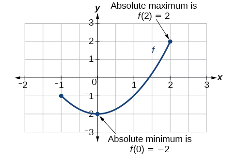
Figure thirteen.

Not every function has an absolute maximum or minimum value. The toolkit function[latex]\,f\left(ten\right)={x}^{3}\,[/latex]is one such office.

Absolute Maxima and Minima

The absolute maximum of[latex]\,f\,[/latex]at[latex]\,x=c\,[/latex]is[latex]\,f\left(c\right)\,[/latex]where[latex]\,f\left(c\right)\ge f\left(x\right)\,[/latex]for all[latex]\,ten\,[/latex]in the domain of[latex]\,f.[/latex]

The absolute minimum of[latex]\,f\,[/latex]at[latex]\,ten=d\,[/latex]is[latex]\,f\left(d\right)\,[/latex]where[latex]\,f\left(d\right)\le f\left(x\right)\,[/latex]for all[latex]\,x\,[/latex]in the domain of[latex]\,f.[/latex]

Finding Absolute Maxima and Minima from a Graph

For the function[latex]\,f\,[/latex]shown in (Figure), find all absolute maxima and minima.

Fundamental Equations

Average charge per unit of alter

[latex]\frac{\Delta y}{\Delta x}=\frac{f\left({x}_{2}\correct)-f\left({x}_{1}\right)}{{ten}_{2}-{x}_{1}}[/latex]

Key Concepts

• A rate of change relates a change in an output quantity to a change in an input quantity. The average rate of modify is determined using but the outset and ending data. See (Effigy).
• Identifying points that marker the interval on a graph can exist used to discover the average rate of change. See (Figure).
• Comparison pairs of input and output values in a table can likewise be used to find the boilerplate rate of alter. Meet (Effigy).
• An average rate of change can besides exist computed by determining the function values at the endpoints of an interval described by a formula. Meet (Effigy) and (Figure).
• The average rate of change can sometimes be determined as an expression. Come across (Figure).
• A function is increasing where its rate of change is positive and decreasing where its rate of change is negative. See (Figure).
• A local maximum is where a function changes from increasing to decreasing and has an output value larger (more than positive or less negative) than output values at neighboring input values.
• A local minimum is where the role changes from decreasing to increasing (every bit the input increases) and has an output value smaller (more negative or less positive) than output values at neighboring input values.
• Minima and maxima are too called extrema.
• We tin can observe local extrema from a graph. See (Figure) and (Figure).
• The highest and lowest points on a graph indicate the maxima and minima. See (Figure).

Section Exercises

Verbal

Can the average rate of change of a function exist abiding?

Bear witness Solution

Yes, the average rate of change of all linear functions is constant.

If a part[latex]\,f\,[/latex]is increasing on[latex]\,\left(a,b\correct)\,[/latex]and decreasing on[latex]\,\left(b,c\right),\,[/latex]then what tin can be said about the local extremum of[latex]\,f\,[/latex]on[latex]\,\left(a,c\correct)?\,[/latex]

How are the accented maximum and minimum similar to and dissimilar from the local extrema?

Show Solution

The absolute maximum and minimum relate to the unabridged graph, whereas the local extrema chronicle only to a specific region around an open interval.

How does the graph of the accented value function compare to the graph of the quadratic office,[latex]\,y={x}^{2},\,[/latex]in terms of increasing and decreasing intervals?

Algebraic

For the following exercises, observe the average rate of change of each function on the interval specified for real numbers [latex]\,b\,[/latex]or[latex]\,h[/latex] in simplest form.

[latex]f\left(x\right)=4{x}^{two}-7\,[/latex]on[latex]\,\left[ane,\text{ }b\right][/latex]

Show Solution

[latex]iv\left(b+1\right)[/latex]

[latex]yard\left(x\right)=ii{x}^{2}-9\,[/latex]on[latex]\,\left[4,\text{ }b\right][/latex]

[latex]p\left(10\correct)=3x+iv\,[/latex]on[latex]\,\left[ii,\text{ }2+h\right][/latex]

[latex]k\left(x\right)=4x-ii\,[/latex]on[latex]\,\left[iii,\text{ }3+h\right][/latex]

[latex]f\left(x\right)=2{ten}^{2}+one\,[/latex]on[latex]\,\left[x,x+h\right][/latex]

Testify Solution

[latex]4x+2h[/latex]

[latex]g\left(x\right)=3{x}^{2}-two\,[/latex]on[latex]\,\left[x,ten+h\right][/latex]

[latex]a\left(t\right)=\frac{1}{t+four}\,[/latex]on[latex]\,\left[nine,9+h\right][/latex]

Prove Solution

[latex]\frac{-1}{thirteen\left(xiii+h\correct)}[/latex]

[latex]b\left(ten\right)=\frac{1}{x+3}\,[/latex]on[latex]\,\left[1,one+h\right][/latex]

[latex]j\left(x\right)=3{x}^{3}\,[/latex]on[latex]\,\left[1,ane+h\correct][/latex]

Testify Solution

[latex]3{h}^{two}+9h+nine[/latex]

[latex]r\left(t\correct)=4{t}^{three}\,[/latex]on[latex]\,\left[2,2+h\right][/latex]

[latex]\frac{f\left(x+h\correct)-f\left(x\right)}{h}\,[/latex]given[latex]\,f\left(ten\right)=2{x}^{2}-3x\,[/latex]on[latex]\,\left[x,10+h\right][/latex]

Evidence Solution

[latex]4x+2h-3[/latex]

Graphical

For the following exercises, consider the graph of[latex]\,f\,[/latex]shown in (Figure).

Estimate the boilerplate charge per unit of alter from[latex]\,x=ane\,[/latex]to[latex]\,10=4.[/latex]

Estimate the average charge per unit of change from[latex]\,ten=2\,[/latex]to[latex]\,x=5.[/latex]

Prove Solution

[latex]\frac{4}{three}[/latex]

For the post-obit exercises, use the graph of each office to estimate the intervals on which the part is increasing or decreasing.

Show Solution

increasing on[latex]\,\left(-\infty ,-2.v\correct)\cup \left(1,\infty \right),\,[/latex]decreasing on[latex]\,\left(-2.5,\text{ }1\right)[/latex]

Show Solution

increasing on[latex]\,\left(-\infty ,1\correct)\loving cup \left(3,4\correct),\,[/latex]decreasing on[latex]\,\left(1,iii\right)\loving cup \left(4,\infty \right)[/latex]

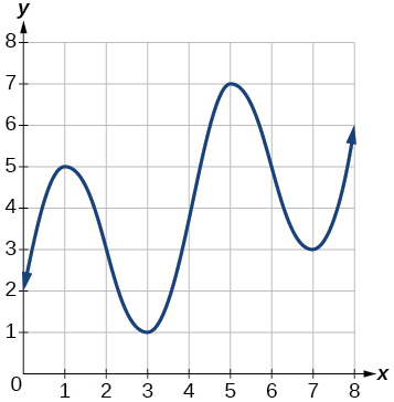
For the following exercises, consider the graph shown in (Figure).

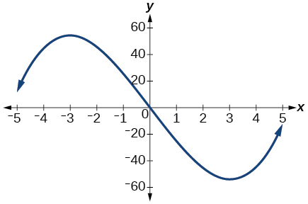
Estimate the intervals where the function is increasing or decreasing.

Estimate the betoken(s) at which the graph of[latex]\,f\,[/latex]has a local maximum or a local minimum.

Show Solution

local maximum:[latex]\,\left(-three,\text{ }60\right),\,[/latex]local minimum:[latex]\,\left(three,\text{ }-60\correct)\,[/latex]

For the following exercises, consider the graph in (Effigy).

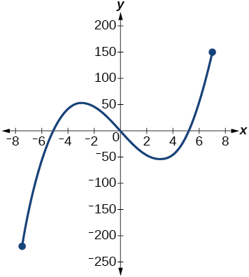
If the consummate graph of the function is shown, estimate the intervals where the role is increasing or decreasing.

If the complete graph of the function is shown, approximate the accented maximum and absolute minimum.

Show Solution

accented maximum at approximately[latex]\,\left(7,\text{ }150\right),\,[/latex]absolute minimum at approximately[latex]\,\left(-7.5,\text{ }-220\right)[/latex]

Numeric

(Figure) gives the annual sales (in millions of dollars) of a production from 1998 to 2006. What was the average rate of change of annual sales (a) between 2001 and 2002, and (b) between 2001 and 2004?

Year	Sales (millions of dollars)
1998	201
1999	219
2000	233
2001	243
2002	249
2003	251
2004	249
2005	243
2006	233

(Figure) gives the population of a town (in thousands) from 2000 to 2008. What was the average rate of modify of population (a) between 2002 and 2004, and (b) between 2002 and 2006?

Year	Population (thousands)
2000	87
2001	84
2002	83
2003	lxxx
2004	77
2005	76
2006	78
2007	81
2008	85

Evidence Solution

a. –3000; b. –1250

For the following exercises, find the average charge per unit of modify of each function on the interval specified.

[latex]f\left(ten\right)={ten}^{two}\,[/latex]on[latex]\,\left[i,\text{ }5\right][/latex]

[latex]h\left(x\right)=5-2{x}^{two}\,[/latex]on[latex]\,\left[-2,\text{4}\right][/latex]

[latex]q\left(10\right)={10}^{3}\,[/latex]on[latex]\,\left[-4,\text{ii}\right][/latex]

[latex]yard\left(x\correct)=3{x}^{three}-1\,[/latex]on[latex]\,\left[-3,\text{iii}\correct][/latex]

[latex]y=\frac{one}{x}\,[/latex]on[latex]\,\left[one,\text{ 3}\correct][/latex]

[latex]p\left(t\right)=\frac{\left({t}^{ii}-iv\correct)\left(t+ane\correct)}{{t}^{ii}+3}\,[/latex]on[latex]\,\left[-3,\text{1}\right][/latex]

[latex]thou\left(t\right)=half-dozen{t}^{ii}+\frac{iv}{{t}^{3}}\,[/latex]on[latex]\,\left[-1,3\right][/latex]

Applied science

For the post-obit exercises, use a graphing utility to estimate the local extrema of each role and to guess the intervals on which the part is increasing and decreasing.

[latex]f\left(x\right)={x}^{four}-4{x}^{3}+5[/latex]

Testify Solution

Local minimum at[latex]\,\left(3,-22\correct),\,[/latex]decreasing on[latex]\,\left(-\infty ,\text{ }3\right),\,[/latex]increasing on[latex]\,\left(3,\text{ }\infty \right)\,[/latex]

[latex]h\left(x\right)={10}^{5}+five{x}^{four}+10{x}^{3}+x{x}^{2}-one[/latex]

[latex]g\left(t\right)=t\sqrt{t+3}[/latex]

Show Solution

Local minimum at[latex]\,\left(-2,-ii\correct),\,[/latex]decreasing on[latex]\,\left(-3,-two\right),\,[/latex]increasing on[latex]\,\left(-2,\text{ }\infty \right)[/latex]

[latex]k\left(t\right)=3{t}^{\frac{ii}{3}}-t[/latex]

[latex]m\left(ten\correct)={x}^{four}+2{x}^{3}-12{x}^{ii}-10x+4[/latex]

Bear witness Solution

Local maximum at[latex]\,\left(-0.5,\text{ }6\correct),\,[/latex]local minima at[latex]\,\left(-3.25,-47\right)\,[/latex]and[latex]\,\left(2.one,-32\right),\,[/latex]decreasing on[latex]\,\left(-\infty ,-3.25\correct)\,[/latex]and[latex]\,\left(-0.5,\text{ }2.1\right),\,[/latex]increasing on[latex]\,\left(-3.25,\text{ }-0.five\correct)\,[/latex]and[latex]\,\left(two.i,\text{ }\infty \right)\,[/latex]

[latex]n\left(10\right)={x}^{4}-eight{x}^{iii}+18{ten}^{two}-6x+2[/latex]

Extension

The graph of the part[latex]\,f\,[/latex]is shown in (Figure).

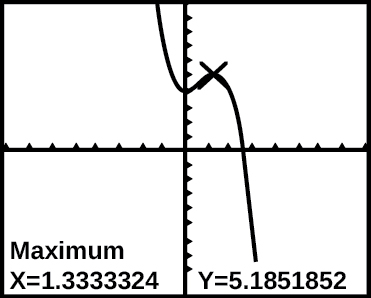
Based on the calculator screen shot, the point[latex]\,\left(1.333,\text{ }5.185\correct)\,[/latex]
is which of the post-obit?

1. a relative (local) maximum of the function
2. the vertex of the function
3. the absolute maximum of the function
4. a nil of the office

Let [latex]f\left(ten\correct)=\frac{1}{x}.[/latex] Find a number[latex]\,c\,[/latex]such that the average rate of change of the function[latex]\,f\,[/latex]on the interval[latex]\,\left(1,c\right)\,[/latex]is[latex]\,-\frac{1}{4}.[/latex]

Let[latex]\,f\left(ten\right)=\frac{1}{ten}[/latex]. Notice the number[latex]\,b\,[/latex]such that the average charge per unit of change of[latex]\,f\,[/latex]on the interval[latex]\,\left(2,b\right)\,[/latex]is[latex]\,-\frac{1}{10}.[/latex]

Show Solution

[latex]b=5[/latex]

Real-Globe Applications

At the showtime of a trip, the odometer on a auto read 21,395. At the end of the trip, 13.five hours later, the odometer read 22,125. Assume the scale on the odometer is in miles. What is the average speed the machine traveled during this trip?

A driver of a car stopped at a gas station to make full his gas tank. He looked at his lookout, and the time read exactly three:twoscore p.m. At this time, he started pumping gas into the tank. At exactly 3:44, the tank was full and he noticed that he had pumped 10.vii gallons. What is the average charge per unit of period of the gasoline into the gas tank?

Show Solution

ii.7 gallons per minute

Almost the surface of the moon, the altitude that an object falls is a office of time. It is given by[latex]\,d\left(t\right)=2.6667{t}^{2},\,[/latex]where[latex]\,t\,[/latex]is in seconds and[latex]\,d\left(t\right)\,[/latex]is in anxiety. If an object is dropped from a certain meridian, find the boilerplate velocity of the object from[latex]\,t=one\,[/latex]to[latex]\,t=2.[/latex]

The graph in (Figure) illustrates the decay of a radioactive substance over[latex]\,t\,[/latex]days.

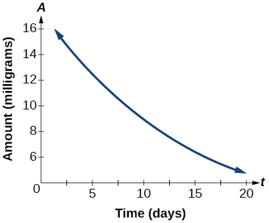
Use the graph to estimate the average decay charge per unit from[latex]\,t=v\,[/latex]to[latex]\,t=xv.[/latex]

Show Solution

approximately –0.half dozen milligrams per twenty-four hour period

Glossary

absolute maximum

the greatest value of a role over an interval

accented minimum

the everyman value of a function over an interval

average rate of alter

the difference in the output values of a function found for 2 values of the input divided by the difference betwixt the inputs

decreasing function

a function is decreasing in some open up interval if[latex]\,f\left(b\right)<f\left(a\right)\,[/latex]for any ii input values[latex]\,a\,[/latex]and[latex]\,b\,[/latex]in the given interval where[latex]\,b>a[/latex]

increasing function

a role is increasing in some open interval if[latex]\,f\left(b\correct)>f\left(a\right)\,[/latex]for any two input values[latex]\,a\,[/latex]and[latex]\,b\,[/latex]in the given interval where[latex]\,b>a[/latex]

local extrema

collectively, all of a function's local maxima and minima

local maximum

a value of the input where a role changes from increasing to decreasing as the input value increases.

local minimum

a value of the input where a function changes from decreasing to increasing every bit the input value increases.

rate of change

the modify of an output quantity relative to the alter of the input quantity

Source: https://courses.lumenlearning.com/suny-osalgebratrig/chapter/rates-of-change-and-behavior-of-graphs/

Posted by: zornrompheight.blogspot.com

Share this post